I enjoyed reading DeepSeek's NSA and I thought it would be an interesting challenge to implement and optimize it for TPUs.

I was especially curious about how NSA, which is heavily optimized for GPUs, could be optimized for TPUs which have fundamentally different design philosophies.

Before we dive in, here's the link to the colab notebook where all my code is. This includes the vectorized JAX baseline of NSA, Pallas kernels, and profiling code. I hope you get to tinker with my code to understand NSA and Pallas better.

Note: All code and experiments ran with TPU v5e. We'll be looking at Selection Branch only as that is the most quirky branch in NSA.

Let me first convince you why NSA is great for GPUs.

Why NSA is Great for GPUs

TLDR: Dynamic sparsity through pointer-based memory loads + High TensorCore Util by Design

1. Dynamic Sparsity

Dynamic sparsity is at the heart of NSA. Recall that NSA first computes the importance score, picks top-K most important blocks, then iterates on those selected KV blocks in the top-K order. In other words, we do not know which blocks to iterate over until we compute the top-K.

This means our hardware must be flexible enough to accommodate this dynamic indexing. And GPUs do this efficiently through pointer-based memory loads.

Also, NSA's top-K operation can be done on GPUs with parallel bitonic sort, thus providing a natural mapping as well.

2. High TensorCore Utilization by Design

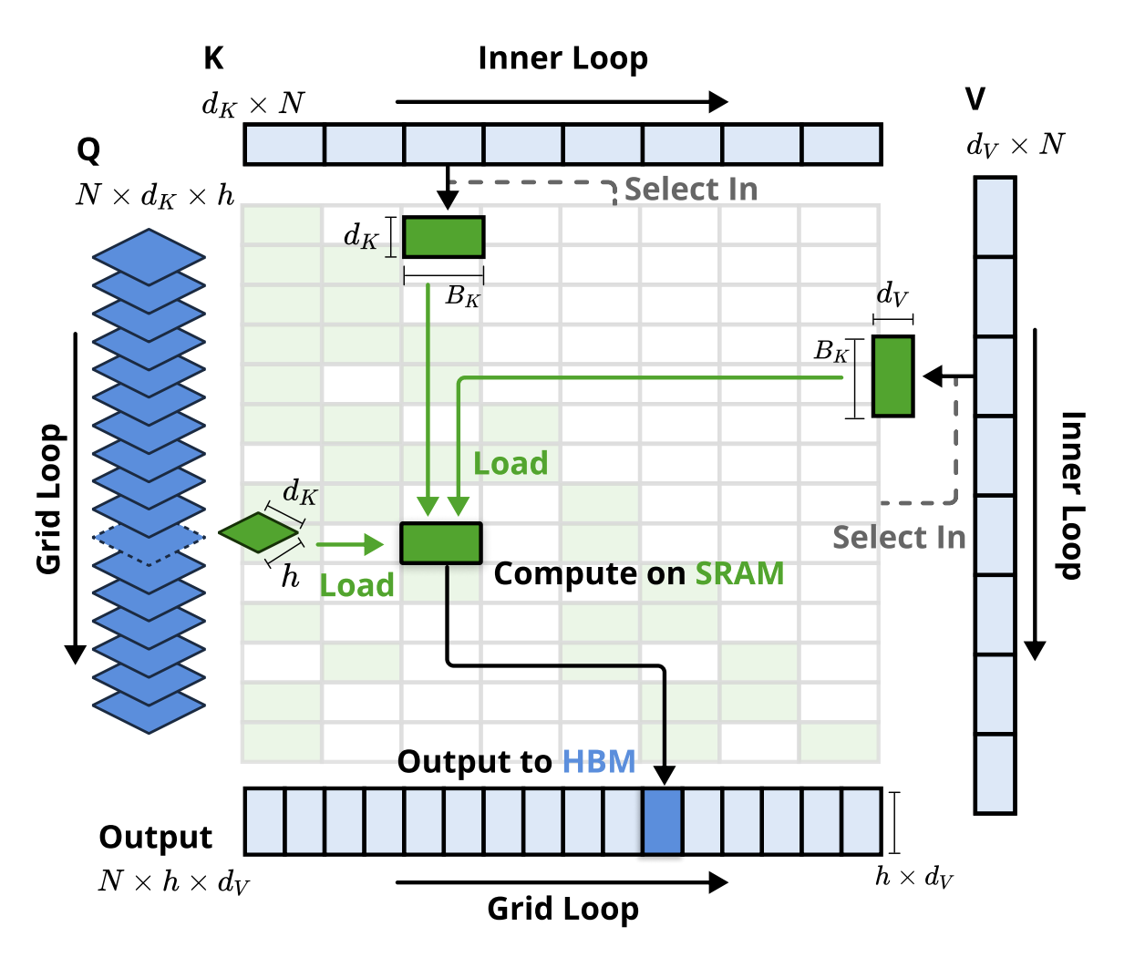
NSA uses a Group Tiling scheme where the outer loop is on the number of GQA groups(i.e. A single query tile is size [G, H] where G is the number of heads per group and H is head dimension).

The original paper talks about memory bandwidth benefits(i.e. coalesced KV block loads since all query heads within a group share KV blocks), but this design extends to systematically preventing GEMVs, therefore increasing TensorCore Utilization.

This is because TensorCores are activated when we at least have dimensions of 8+ and preferably 16+. This means naive query batching without Group Tiling can easily be nerfed to GEMVs instead of GEMMs if a tile is not large enough. Group Tiling systematically prevents this as even a single query batch already has [16, H]@[H,Bk]. This sort of defensive programming is one of the many reasons I like NSA.

But let's now see how this is difficult for TPUs.

Why NSA is Difficult for TPUs

TLDR: We don't have any Pros from the GPU section except the contiguous token blocks.

Dynamic sparsity is quite difficult on all levels of the TPU stack: JAX/XLA, Pallas, and TPUs. Jitted code using JAX/XLA are not friendly towards runtime variables and dynamic branching, which NSA both has. Moreover, Pallas's programming model enforces a fixed, lexicographical traversal through data which is directly unfavorable towards NSA's top-K based dynamic traversal. And finally, TPUs prefer large and dense blocks rather than thin slices.

Now that I'm done complaining, let's dive into the implementation. But before we do so, one small fix is required.

Fixing Equation 9

\[ \mathbf{p}_{t}^{\text{slc}}[j] \;=\; \sum_{m=0}^{\tfrac{l'}{d}-1} \; \sum_{n=0}^{\tfrac{l}{d}-1} \mathbf{p}_{t}^{\text{cmp}}\!\left[\tfrac{l'}{d}j - m - n\right] \]

Equation 9 in the paper has an error. Its purpose is to do block-wise pooling for cases when the block size used in the compression branch differs from that of the selection branch.

However, its index calculations are off and it could also be simplified much further given the assumptions that NSA provides. First, NSA assumes a unified stride value. Secondly, it also assumes a divisibility constraint where block sizes from both branches must be divisible by the stride \((l \bmod d = 0 \text{ and } l' \bmod d = 0)\). This means all blocks – regardless of the branch – are aligned with the stride grid. And concretely, NSA’s original setup follows these assumptions and uses \(d = 16,\; l = 32,\; l' = 64\).

We can rewrite Eq.9 into standard blockwise pooling with this. Here’s the corrected version:

\[ \mathbf{p}_{t}^{\text{slc}}[j] \;=\; \sum_{n=0}^{\left\lfloor \tfrac{\,l'-l\,}{d} \right\rfloor} \mathbf{p}_{t}^{\text{cmp}}[j+n] \]

XLA-Unfriendly JAX Version (Naive)

Before we even start writing kernels, however, we need to verify if one is even needed at all.

The XLA compiler is extremely powerful, such that oftentimes we might be able to get satisfactory performance just by writing good jitted code.

Then what is a bad, XLA-unfriendly code? Non-vectorized code is a common example, but one "gotcha" is XLA-unfriendly indexing. And this is quite common in ML. Let's look at an example of this.

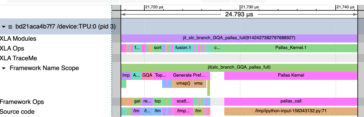
Here's the profile trace for the naive NSA implementation below. We see that "Build K_slc, V_slc" is taking up >99% of the time (Note: sequence length is 2048 for testing).

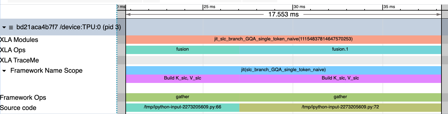
Below is the code responsible for the majority of the trace.

with jax.named_scope("Build K_slc, V_slc"):
   K_slc = K_orig[
       jnp.arange(K)[:, None, None],  # [K,     None, None]
       blk_idx[:, :, None],           # [top_n, l',   None]
       jnp.arange(H)[None, None, :]   # [None,  None, H   ]
   ] # [K top_n*l' H]
                 
   V_slc = V_orig[
       jnp.arange(K)[:, None, None],
       blk_idx[:, :, None],
       jnp.arange(H)[None, None, :]
   ] # [K top_n*l' H]

This seemingly innocent code has an indexing inefficiency. Specifically, each indexing axis(jnp.arange(K), blk_idx, jnp.arange(H)) is broadcasted to shape [K, top_n, l', H] to accommodate all indexes. Even worse, they are then stacked together into a final index tensor of shape [K, top_n, l', H, 3].

This means a large index tensor has to be materialized in our HLO graph, which XLA struggles to optimize.

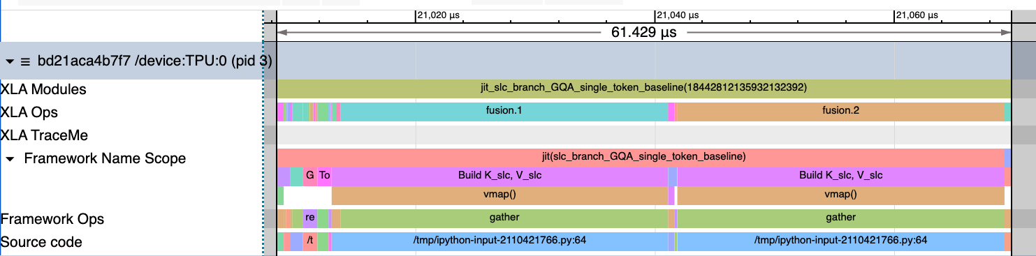
Instead, we can change this to explicitly gather selected elements with vmap:

def gather_slc(idx, orig_mat):
   # orig_mat [K T H]
   # idx      [topn*l' K]
   return orig_mat[jnp.arange(K), idx, :]


 with jax.named_scope("Build K_slc, V_slc"):
   K_slc = jax.vmap(gather_slc, in_axes=(0, None))(blk_idx, K_orig) # [topn*l' K H]
   V_slc = jax.vmap(gather_slc, in_axes=(0, None))(blk_idx, V_orig) # [topn*l' K H]

This small change alone avoids working with the huge index tensor allowing XLA to optimize it well.

However, in reality, if this is a research code with experimental ideas then code readability is significantly more important. Context switching is difficult when you're writing code for correctness versus for performance.

Let's now see if a vectorized and XLA-friendly version performs better than our original.

Vectorized JAX Baseline of NSA's Selection Branch

Vectorizing and performant indexing alone already gives us ~286x performance boost. This is not surprising as clean Gathers can give us speedups of 1~2 orders of magnitude.

But notice how the majority of the time is still spent on building \(K_{\text{slc}}\) and \(V_{\text{slc}}\) matrices. Moreover, it's also spiking memory usage as these matrices are materialized.

This necessitates the need for a fused kernel for the following reasons:

1. Unnecessary memory burden for materializing \(K_{\text{slc}}\), \(V_{\text{slc}}\)

- We only need \(K_{\text{slc}}\), \(V_{\text{slc}}\) to get the output, \(O_{\text{slc}}\)

- Even if we might need them, it's faster to rematerialize them on the fly than to be memory BW bound

2. XLA's Gather op runs on VPUs and is memory BW bound

- A rule of thumb for TPUs is to maximize MXU ops and minimize/overlap VPU ops.

Fusing is a good point to start. But to do this, we need to introduce Pallas, the JAX kernel language.

TPU Pallas Introduction

Pallas is the kernel language for JAX. It's still an experimental framework and it's an interesting mix of Triton and JAX.

One key characteristic of Pallas is using tiles as natural units. I like this a lot since unlike graphics, tiling serves as the universal intuition behind ML: we think in terms of blocked MMA, coalescing blocked memory loads, and so on.

Aside: Tiling Philosophy Trends

Tiling philosophy is not unique to TPUs; ThunderKittens also uses 16x16 tiles as natural units. Moreover, newer Blackwell GPUs may actually prefer this paradigm more since their TensorCores are growing larger.

Let's dive into Pallas now. One key quirk of Pallas is that it also brings in the functional nature of JAX into kernel programming. This is better seen than said, so let's look at a matmul example in Pallas below.

There are two key pieces:

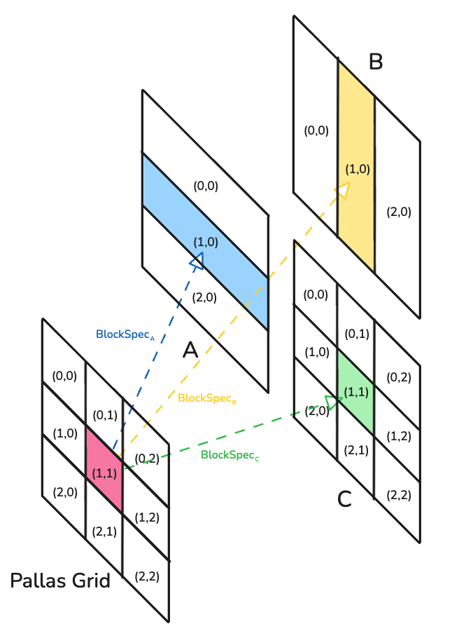
Grid
- Program ID of each kernel (i.e. number of subproblems or kernels launched)

BlockSpec
- Defines which section of the array is relevant for a given grid indice(i.e. program ID).

Hence, TPU programming can be seen as a mapping and dataflow problem where your job is to find the optimal data sharding that consistently feeds streams of data to the systolic arrays(MXU).

However, recall that NSA is sparse. Then how do we deal with sparsity in Pallas TPU?

Dealing with Sparsity in Pallas TPU

We can use the Scalar Prefetch feature in Pallas.

TLDR on Scalar Prefetch: Pipeline optimization -- Don't load data that's not used.

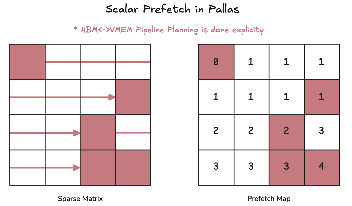
We can divide along the sequence dimension and only select blocks that are selected by top-K.

However, there is a problem with traversal order.

Issue 1: Non-Monotonic Top-K Traversal

The original NSA algorithm's selection branch first selects top-k blocks and then chooses to traverse through \(K_{\text{orig}}\), \(V_{\text{orig}}\) in the order of top-k blocks. This means that we won't have sorted block indices. This is not a problem on GPUs as each kernel can be assigned a block and memory accesses can be done in parallel.

Such is not the case for the TPU. Recall that TPUs are closer to highly sequential chips and the Pallas programming model reflects this. In fact, Pallas enforces this by iterating through the grid in lexicographical order, thus restricting any access to previous grid blocks. This has direct implications on the original algorithm as we can't traverse the top-k selected blocks if they are not monotonically increasing(e.g. top_k_indexes = [7,6,1,2] traversal goes against Pallas programming model).

The solution lies in softmax's order invariant property.

Solution: Use Order Invariance of Online Softmax

\[ \begin{aligned} &\textbf{for } i = 1 \;\text{ to } \#\text{tiles do} \\ &\quad x_i = Q[k,:] \; K^{T}[:, (i-1)b : ib] \\ &\quad m_i^{(\text{local})} = \max_{j=1}^{b} \big( x_i[j] \big) \\ &\quad m_i = \max \big( m_{i-1},\; m_i^{(\text{local})} \big) \\ &\quad d_i = d_{i-1} \, e^{m_{i-1} - m_i} + \sum_{j=1}^{b} e^{\,x_i[j] - m_i} \\ &\quad o_i = o_{i-1} \, e^{m_{i-1} - m_i} + \sum_{j=1}^{b} e^{\,x_i[j] - m_i} \, V[j + (i-1)b, :] \\ &\textbf{end} \\ & O[k,:] = \frac{o_{N/b}}{d_{N/b}} \end{aligned} \]

Online softmax is order invariant. Specifically, it does not matter which order we traverse or process our blocks in. This allows us to reduce the original problem of dynamic, non-monotonic top-k indexing into a normal sparse attention problem. We can simply sort the selected blocks and traverse in that order. And sorting is affordable as its only done on top-n elements, where top-n is extremely small (e.g. NSA paper used top_n=16).

This works as intended on our BF16 (with FP32 accumulation) kernel, but has important numerical stability implications in lower dtypes (especially FP8 and below).

Aside: Is Online Softmax Truly Order Invariant?

Online softmax may seem order invariant, but order matters especially for lower dtypes.

Let's assume the worst-case scenario where variance in attention scores are large(i.e. difference between largest selected block and smallest selection block is large).

Case 1: Descending Order Traversal (original NSA)

This is generally more numerically stable. The global maximum is encountered early, which means subsequent iterations avoid renormalizations. Also, the scaling factor \(\alpha = \exp(m_{\text{prev}} - m_{\text{curr}})\) remains at 1 and all exponentials are bounded by 1 since \(\exp(x - m_{\max}) \leq 1\).

The only issue is underflow due to \(\exp(x - m_{\max})\) resulting in an exponential with a large negative argument. This is not an issue for FP32/BF16, but for FP8/FP4 this will frequently result in underflow and thus “wipe out” previous output accumulations.

However, this is still ideal as it avoids underflow for the largest score, thus resembling a kind of one-hot encoding of softmax. This is to say that it still preserves the purpose of softmax: allocating high scores for important blocks.

Case 2: Ascending Order Traversal

This is the opposite scenario. Each block includes a new maximum, so we're systematically forced to apply renormalization at each step where \(\alpha = \exp(m_{\text{prev}} - m_{\text{curr}}) < 1\). This repeated downscaling could lead to vanishing values. This isn't ideal, as we have mechanisms to protect against overflow (i.e. \(\exp(m_{\text{curr}} - m_{\text{global}})\)), but not against underflow.

This case is especially worse for FP8/FP4 as we might "wipe out" accumulated results before we reach the maximum, which is the value we want to assign as the highest softmax score.

The main distinction between the two cases is whether underflows meddle with our original purpose of softmax or not.

This is why the design of intermediate accumulation and renormalization requires careful codesign of three factors: dtype choice, renormalization timing (per-step or at the end), block size, and total sequence length(i.e. Total number of tiles).

Experiment Proposal:

An interesting experiment would be to show a sequence length(8K ~ 1M) vs error accumulation plot with 4 lines(1. BF16 & single normalization, 2. BF16 & per-step normalization, 3. FP8 & single normalization, 4. FP8 & per-step normalization). Another plot could be the same but with differing tile sizes. This won't be trivial since different hardware makes different choices in which dtypes to use to accumulate specific operations, thus careful tracking is required. Moreover, experiments with longer sequence length will also have to factor dtypes for reduction operations(e.g. reduce-scatter) across multiple chips.

For our purposes of a BF16 kernel with accumulations done in FP32, however, we can happily use order invariance of online softmax and move on.

But now there's a new challenge: dealing with NSA's strided blocks where many elements overlap between contiguous blocks.

Issue 2: Working with Overlapping Blocks in Pallas is Hard

Let's define the problem first. Assume the worst case scenario where all selected block indexes are contiguous. This becomes an issue because of two reasons:

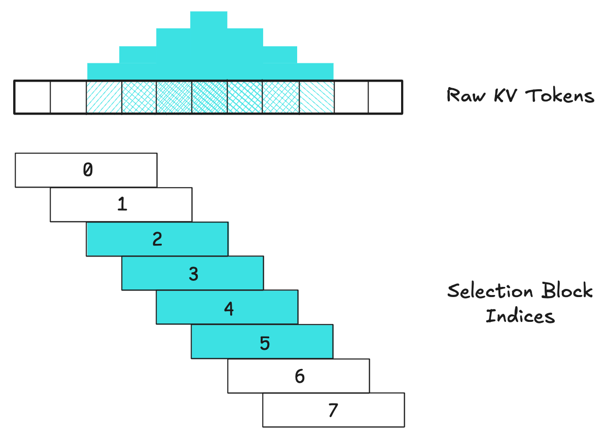
1. Redundant Memory Accesses

- Nearby blocks will share a lot of common elements as stride is less than block size (e.g. Per NSA’s paper setup, contiguous blocks share ¾ elements, which is a significant overlap)

- If each block is fetched independently, however, there will be multiple fetches of the same elements, deteriorating arithmetic intensity.

2. Ambiguous Pallas Grid Definition

- A Grid in Pallas is, by definition, sequential blocks of memory that do not overlap each other.

- This directly conflicts with NSA’s sliding-convolution-esque approach where \(d < l'\).

Changing the stride to be equal to block_size is not an option. Doing this changes the algorithm completely as NSA benefits from information granularity given from overlapping blocks.

In essence, we need to find a way to do strided computation efficiently using Pallas.

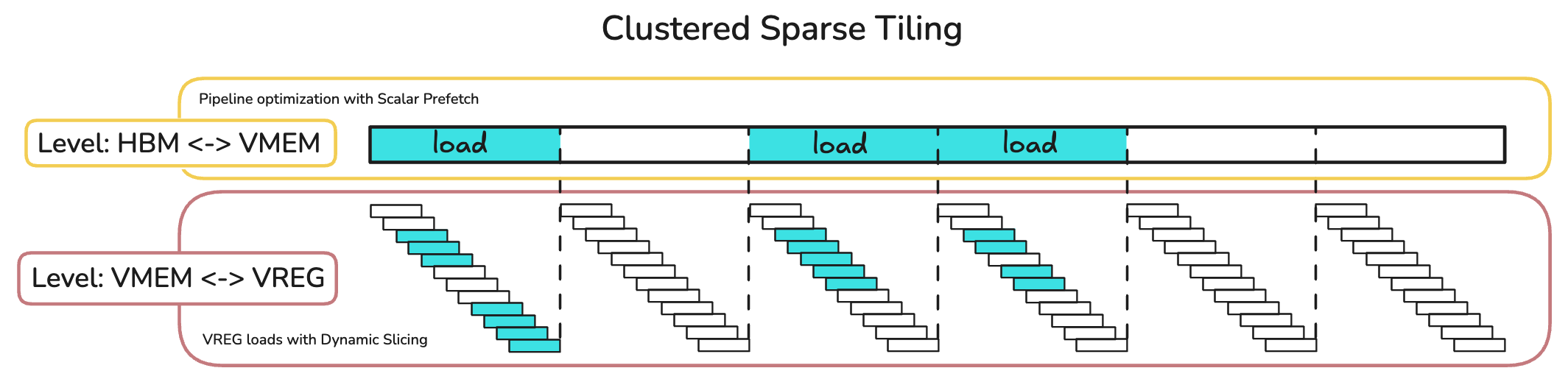
Solution: Clustered Sparse Tiling

My approach is to combine three ideas:

NSA's Spatial locality bias of selected blocks
Leverage larger VMEM of TPUs
Easy pipeline optimization of Pallas

Concretely, NSA's inductive bias is that there is spatial continuity and locality in attention patterns. This extends to the selection branch as selection score distributions follow this blockwise clustering behavior.

We can use this bias directly to optimize pipeline efficiency. Given that one tile of loaded data covers one cluster of selected blocks, we can skip the loading of most tiles. This is allowed as contiguous blocks have high levels of overlap (e.g. \((l' > d;\; l' = 64,\; d = 16)\)).

With NSA's default configuration of \(l' = 64,\; d = 16,\ \text{top_n} = 16\), let's think about the worst-case scenario.

What is the worst-case tile length? (i.e. largest tile)

The worst-case scenario is when all top_n blocks lie in a single cluster(i.e. All top_n blocks are contiguous). Since there is 75% overlap between contiguous blocks, all 16 blocks will lead to a tile size of (64*0.25 * 16) = 256. This will be the upper bound of our Bk dimension where Bk is the tile size used for online softmax.

Recall that at one step we have q[G,H], K[H,Bk], V[H,Bk] of data per query in SRAM. That means we have ([16 * 128] + [128 * 256] + [128 * 256]) * 2(bf16) = 135KiB in SRAM. This is without query batching, so it's a bit large for GPUs, but TPUs have larger VMEMs that can afford multiple batches of this (Note: GPUs can afford pointer-based memory accesses, so this approach is actually not necessary for them).

Tying this into pipeline optimization, all expensive HBM <=> VMEM transfers can be minimized to load only select tiles and skip the rest. And within each loop, each block within a tile has to be loaded sequentially but this is within the VMEM<=>VREG regime which is much faster.

Q. What does a "VREG load with Dynamic Slice" mean?

TPU data movement visualized — Pipelined Pointwise Operation (from "How to Scale Your Model" [9])

This is an interesting combination of how TPU memory pipelining is done on both the hardware and software level.

On the hardware level, TPU memory transfers are done in this order: HBM⇔VMEM⇔VREG⇔MXU/VPU. And Pallas provides an interesting abstraction where it pipelines the transfer of data from HBM⇔VMEM according to our scalar prefetch map before our kernel starts.

This means that we can assume our relevant input tiles(a.k.a Ref; e.g. q_ref) are already living on the VMEM when we write our kernel. When we call q_ref[:] within our kernel, that’s when a copy from VMEM⇔VREG is initiated.

However, we can use dynamic slicing on Refs to avoid copying the entire input tile to VREG, hence the “dynamically sliced VREG load”.

There are some caveats to this. Due to compiler restrictions, although the starting indices of your slice can be dynamic(i.e. runtime variables), your slice size must be static(i.e. compile time constants).

In the case of NSA, we are able to do this as our slice size is the selection block size, which is a fixed parameter.

Given this context, there's an interesting question to be asked: what is the "optimal" tile size?

Finding the Optimal Tile Size for Clustered Sparse Tiling

The naive approach is to run autotuning with different tile sizes, but a good answer is more nuanced due to NSA's dynamic sparsity.

We can use some quirks of NSA to pick the optimal tile size. First, NSA implies that many of their selected blocks will be clustered together (i.e. non-uniform distribution of selected blocks). This means we could very much skip most tiles since most of our selected blocks will be within a couple tiles. But, at the same time, we want each tile to be large enough such that it holds multiple selected blocks due to clustering.

There's three approximate scenarios:

1. \(T < X\): Redundant memory accesses

2. \(T \gg X\): Large pipeline bubbles + low arithmetic intensity

3. \(T \approx X\): Ideal tile size where a single fetch contains one cluster

In essence, this becomes a question of finding the smallest tile size that is still large enough to contain the expected size of a single block cluster.

You might have noticed that knowing the distribution of the attention scores of \(p_{\text{slc}}\) is very important to get a good answer for this. This is true: the optimal tile size may be different depending on the spread of attention scores, locality of block cluster sizes, and also data modality. This is without, of course, harming pipeline efficiency or arithmetic intensity.

This is an example of why I believe large scale ML in the modern day is a full stack problem that no engineer or researcher can do alone. There's quite a lot of moving parts going on. And for natively-trained sparsity approaches like NSA, multiple pretraining runs are probably required just to explore and understanding what best approaches forward may be.

For now, we'll abstract this complexity away and just run with the blockwise-locality assumption that DeepSeek suggested.

Now we just have one more important step: generating the correct prefetch maps for an optimized pipeline performance.

Efficient Prefetch Map Generation with Prefix Scans

Efficiently generating a prefetch map for NSA is a difficult task in itself. This is mostly because of the dynamic sparsity of NSA along with the backward dependency of prefetch maps(i.e. we need to know in advance which blocks to fetch). So a naive implementation of this would be a nested for loop with reversed indexing due to the backward dependency. This would be expensive even considering the fact that a prefetch map is only generated once.

However, we could transform this seemingly sequential problem into a parallel one by spotting the associativity. For each position, instead of asking what the next valid position to fetch is, we can instead ask what the minimum of all valid positions to the right is.

We can now see this as a suffix minimum problem that can be solved with prefix scan on flipped arrays where our binary associative operator is minimum between the two operands.

This approach the added advantage of mapping well to JAX: there's a jax.lax primitive for prefix scans(i.e. jax.lax.associative_scan) and is easily vmap-able, extending it for batched GQA heads or batched queries.

This covers prefetch maps for a dense-grid case, but recall that we're working with a sparse grid for NSA. This is to say whenever we don't want this tile, we should avoid loading it at all.

We can use sentinels to solve this. In essence, we flag invalid indices(i.e. tiles we skip) with sentinels to prevent them from interfering with our scan operation.

Aside 1: Avoid `jnp.inf` as Sentinels

I also ran into an interesting case with using jnp.infs as my sentinels: my HLO traces were being unnecessarily cluttered due to this small choice. This was because the compiler had to add extra conversion steps to accommodate both integer indices and my infinity which was represented as a floating point. Here’s one snippet below:

fused_computation.17 {
  param_1.207 = s32[4,256]{1,0:T(4,128)S(1)} parameter(1)
  convert.4 = u16[4,256]{1,0:T(4,128)(2,1)S(1)} convert(param_1.207)
  …
  broadcast.87 = f32[4,256]{1,0:T(4,128)} broadcast(param_0.153), dimensions={1}
  constant.124 = f32[]{:T(128)} constant(inf)
  broadcast.86 = f32[4,256]{1,0:T(4,128)} broadcast(constant.124), dimensions={}
  select.30 = f32[4,256]{1,0:T(4,128)S(1)} select(compare.36, broadcast.87, broadcast.86)
  ROOT tuple.1 = (f32[4,256]{1,0:T(4,128)S(1)}, u16[4,256]{1,0:T(4,128)(2,1)S(1)}) tuple(select.30, convert.4)
}

The constant, broadcast, select ops had to be added just to accommodate my choice of jnp.inf. I left it as is now since I thought this doesn't increase my runtime(just increasing the time taking to compile), but got me curious whether large scale production systems consider this a problem.

Aside 2: Practical Implementation Notes

This approach of generating prefetch maps is, ironically, more fit for GPUs than TPUs as GPUs can leverage parallel execution models for doing parallel scans. Also, scan operations on TPUs burden VPUs, which we generally don't want especially when prefetch arrays get very long. So careful attention should be spent on overlapping the prefix map generation with computation(i.e. Construct the prefix map for batch i+1 while computing batch i).

Now, let's look at the results.

Results

1. Vanilla case for seqlen=2048; Single Query

There's a ~2.5x speedup and an approximately (K * num_slc_blks*slc_blk_size * H * 4(FP32) * 2(for K_slc, V_slc) reduction in memory, as these intermediate matrices are no longer materialized.

As a disclaimer this is definitely cherry-picked and this trend does not continue for long sequences. We'll analyze this shortly after, but let's check correctness first.

2. Correctness

This passes a jnp.allclose with our baseline using rtol=1e-6, atol=1e-4 with input/outputs in BF16. This was made possible because our online softmax and matmul accumulations were done in FP32.

Here's a summary plot I used a lot for debugging while coding the kernel:

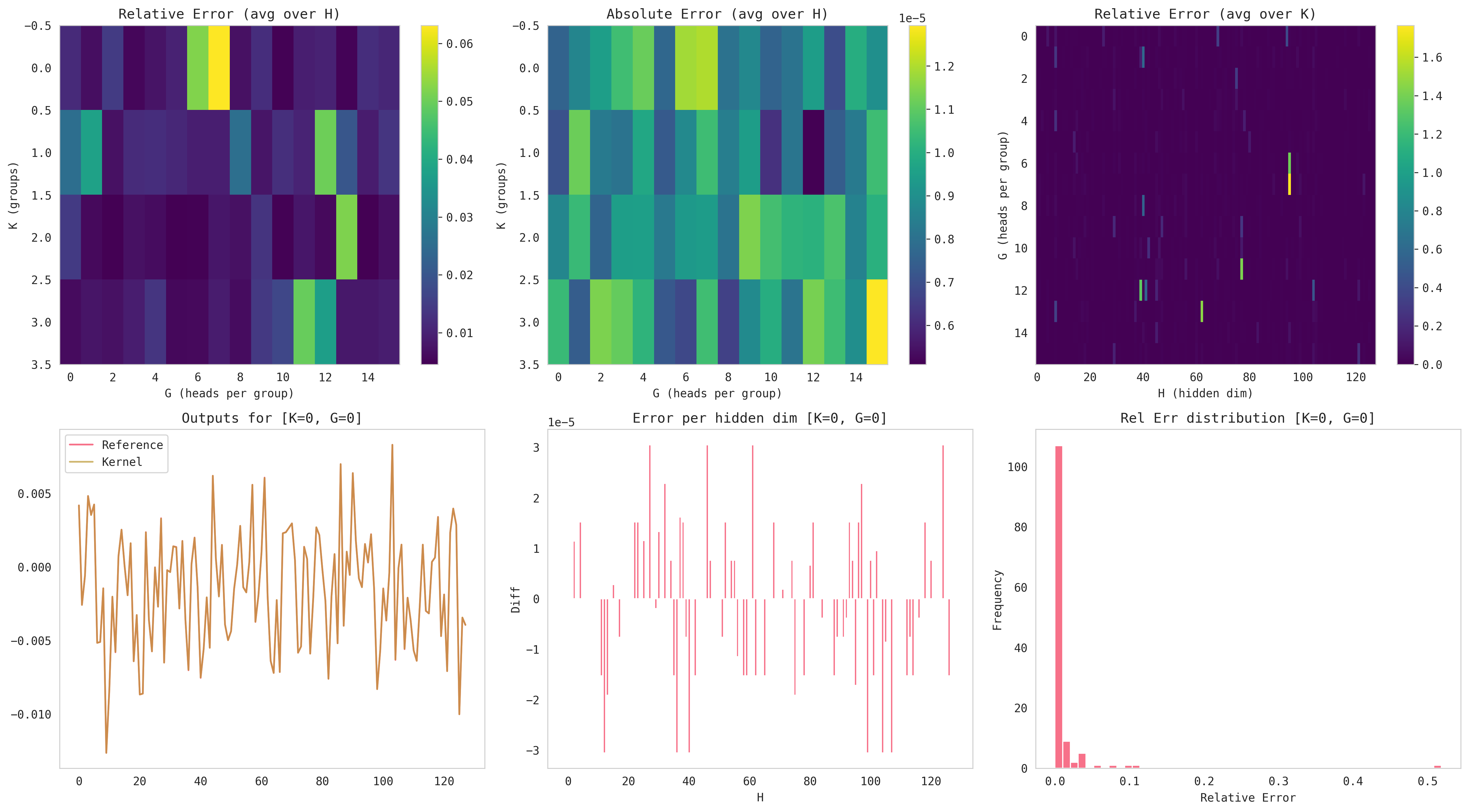
For our case, the absolute error is most relevant since our synthetic test data was initialized with a standard normal distribution (Note: low variance centered around zero makes rtol spikes more likely; but atol for these elements are typically low, thus passing jnp.allclose).

Aside: Visualization Tooling Matters

Debugging numerical stability issues would have been significantly more difficult without these plots. More time spent visualizing allowed debugging much easier and I'm curious what tools performance people in industry have to visualize the data and trace better.

Note: Treescope was a great tool to visualize matrices as well!

Let's go back to benchmarking. Previously, we've only tested a vanilla case for a short sequence length of 2048.

Although it's a bit premature to benchmark long context without query batching implemented, let's see how it does.

3. Long Context Performance (...but only Single Query for now)

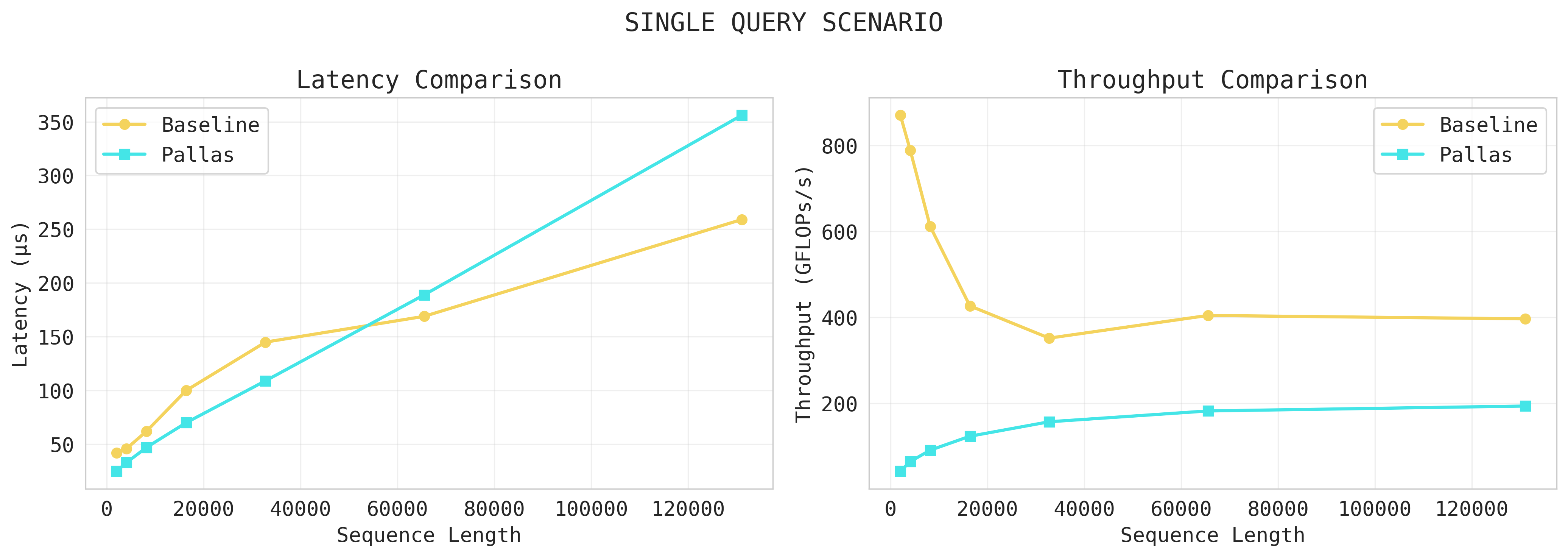
My kernel does not scale for long contexts and severely underuses hardware. Let's think about why this is the case. The easy way out would be to say this because we're only doing single-query, but there's more nuances when we dig in.

First, let's analyze the obvious culprit:

1. MXU / VPU Underutilization

Arithmetic intensity is quite low as our kernel is closer to a GEMV than a GEMM in a single-query scenario. Recall that TPUs perform matmuls on MXUs, which are 128x128 systolic arrays(newer TPUs have 256x256). Specifically, they perform a single [8x128]@[128,128] matmul per 8 cycles.

However, recall that our kernel's single query case is doing
q_tile[G,H] @ K_blk[slc_blk_size, H].T = [16,128]@[128,128]. This is essentially a GEMV-esque operation on a TPU since this is done in 16 cycles. In other words, the "stream" of data that systolic arrays love is absent.

Also, the way we handle VPU ops is problematic too. Any vector operation(i.e. online softmax operations) are done by VPUs, and they specifically want (8,128) tiles. However, our current online softmax accumulators are in [G, 1]=[16,1]. This means that each accumulator has to be padded to [16,256] to be passed into our VPU, hence limited by VPU bandwidth. Thus, VPU lane optimization must be done when implementing query batching.

However, there's a more subtle experiment-setup issue:

2. Inductive Bias Not Reflected in Synthetic Data

Recall that our inductive bias for this kernel design was assuming that blocks will be clustered together as the NSA paper implies. This is, however, not reflected well in our synthetic data.

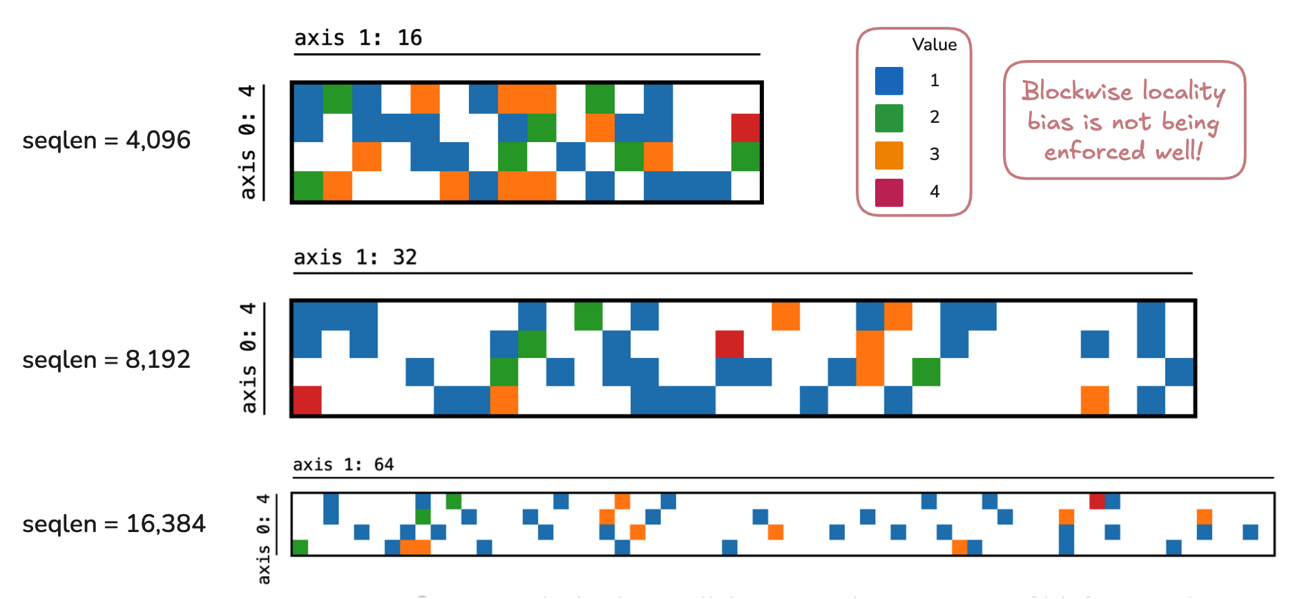
Above are the prefetch maps of three sequences(\(\text{top-}n = 16\)). Ideally, we want to see most blocks clustered into a few chunks for each row. Instead, however, we only have 1~2 blocks per chunk.

This means we have a terrible pipeline where most chunks will be loaded to process just 1~2 blocks, hence deteriorating arithmetic intensity.

I initialized our data with standard normals, then injected topic vectors to emulate sparsity. My topic vectors have some effect(as seen by occasional orange and red squares), but clearly not enough to emulate NSA's blockwise-clustering bias.

It left me wondering: "What do the attention distribution patterns in a fully trained NSA look like?" and "How can we use that to design more efficient kernels?". I'm curious if there's a direction of "distribution-aware" kernel designs.

This is partly why I was stuck on coming up with a good query batching scheme for NSA that’s fit for TPUs. Since each query dynamically selects a different set of selection blocks, a naive query batching scheme will most-likely lead to large pipeline inefficiencies.

There’s some puzzle pieces in my head about whether we could use some blockwise-locality pattern to design a variant of “union query tiling”(i.e. Queries in a batch share the same or nearby KV chunks). However, I think this will be heavily dependent on the attention distribution pattern or the actual training dynamics of NSA.

But to return to some concrete things again, here’s a final list of miscellaneous optimization and next steps to take.

Miscellaneous: SMEM Memory Optimization

We can store scalar prefetch args in uint16 to save SMEM space and upcast on the fly.

Although modern TPUs have SMEM sizes of ~1 MiB which does not necessitate this, I was originally working with TPUv2s that have a SMEM capacity of 16 KiB, hence the fix.

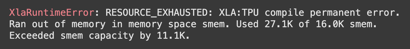
Specifically, when I was testing with \(\text{seqlen} = 131{,}072;\; B_k = 256;\; \text{top_n} = 16\), the total size of our scalar prefetch args alone is 24.8 KiB ((compute_mask[K, T_kv//Bk] + prefetch_map[K, T_kv//Bk] + compute_base_idx[K, T_kv//Bk] + global_slc_idx[K, top_n]) * 4(FP32)) = 24.832 KiB).

We can do a small optimization of storing the compute_mask, prefetch_map, and compute_base_idx in uint16 and upcast to int32 as needed (Note: indexes must be int32 in Pallas, so upcasting is a necessity).

The global_slc_idx should be kept at int32 as the representable range of uint16 is [0, 65,536) and, thus is not able to accommodate indices for long sequences. For a similar reason, downcasting other arguments to uint8 is not possible as it leads to integer overflow.

This reduces our total SMEM usage to 12.54 KiB (3*(K * T_kv//Bk) * 2(uint16) + (K * T_kv//Bk) * 4(FP32) = 12.544 KiB).

Current Limitations and Next Steps

1. Fix Block Stride Edge Case

My current kernel has a critical edge case: it does not account for when selection blocks lie between the fixed boundary of two tiles.

- Potential approach: User 'rdyro' from JAX discord suggested using manual DMA from HBM to design my own memory pipeline.

2. Changing Selection Block Size, Compression Block Size, and Stride

Although my NSA JAX baseline uses the default setting \((l = 32,\; l' = 64,\; d = 16,\; \text{top_n} = 16)\) from the NSA paper, my TPU kernel implementation uses slightly different values\((l = 64,\; l' = 128,\; d = 32,\; \text{top_n} = 8)\).

This was to accomodate for hardware utilization(e.g. MXU layout is 128x128), token budget consistency(keep slc_blk_size * top_n consistent), and information overlap granularity (keep overlap factor for contiguous selection blocks to be ¾).

However, this could change training dynamics completely as the same fine-grained information may be lost. For example, a smaller selection block size may allow the model to extract only a few tokens around the "important" part whereas a large selection block size may also include irrelevant tokens.

My guess is that this could lead the model to be less performant on fine-grained recall tasks(e.g. needle in a haystack) where a smaller token block may be advantageous.

3. Design an Effective Query Batching Scheme

Query batching has two large issues to think about:

a. Overhead of computing prefetch maps due to dynamic sparsity

b. Naive query batching does not guarantee a sparse prefetch map(e.g. worst case: query 0 ~ 16 could each select top_n number of selection blocks where no overlaps occur).

The idea of union query tiling I was thinking above came from wondering whether if there's a way we can batch queries that attend to similar selection blocks. If so, then we could take the union of necessary selected blocks and find optimal tile sizes based on this. But this seemed like a stretch, especially without looking at concrete attention distributions. I'll have to give this more thought, but please help me out if you have any ideas!

Closing

This was a fun project to work on, and it was a lot more challenging than I expected. I titled this as a "worklog", but this is actually kernel iteration 1, so I'll continue to look at this. I want to explore distribution kernels next too since I think those are scenarios where TPUs can shine even more.

Until then, I hope this blog and the colab notebook helps others tinker with TPUs and Pallas.